In the previous tutorials we learned how to create plots and display them in a Jupyter notebook. But how can we share them outside of a notebook?
In this tutorial we cover how to save plots so they can be shared/used in reports, and how to display them in a Streamlit app.
Saving figs: Matplotlib
You can save your plot as a file to disk using matplotlib’s savefig function. The function takes as its first argument a string specifying the full path (including the filename) of the file to create. Multiple file formats are supported (e.g., png, jpeg, pdf, svg); png is most commonly used. The file format is inferred from the file name extension. For example, if you save your figure to plot.png, the figure will be saved as a png file.
The savefig function is actually a method of the figure object. As with creating plots, you can save figures either via the explict object-oriented way (my preferred way) or via stateful execution.
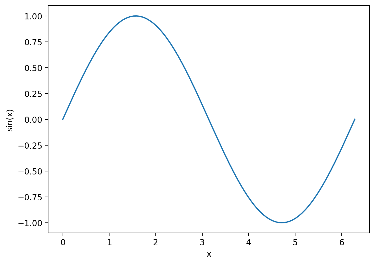
import numpy as npfrom matplotlib import pyplot as plt# create the datax = np.linspace(0, 2*np.pi, 100)y = np.sin(x)# plot itfig = plt.figure()ax = fig.add_subplot()ax.plot(x, y)ax.set_xlabel('x')ax.set_ylabel('sin(x)')
Text(0, 0.5, 'sin(x)')
Now to save it (here, as a png):
fig.savefig('sine.png')
The savefig argument also takes other arugments. One of the most common to use is dpi. This sets the resolution of the plot. The default is based on your system settings, but is typically 100 dots/inch. This can sometimes be too pixelated, especially if you are embedding the plot in a document that you wish to print. Set dpi=300 for typical publication-quailty pngs.
Stateful way
The same code above, but using stateful execution:
import numpy as npfrom matplotlib import pyplot as plt# create the datax = np.linspace(0, 2*np.pi, 100)y = np.sin(x)# plot itplt.plot(x, y)plt.xlabel('x')plt.ylabel('sin(x)')# save itplt.savefig('sine.png')
Saving figs: Seaborn
Seaborn, being built on top of matplotlib, just uses matplotlib’s savefig method to save plots. To do that you can explicitly get the figure using the get_figure() method. This method can be called on the objects returned by a Seaborn plotting command (which are actually returning matplotlib Axes instances).
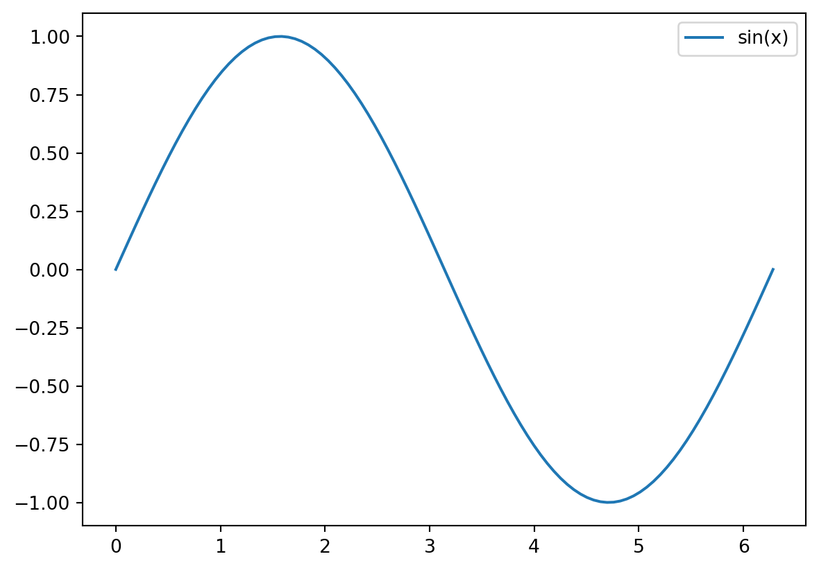
Repeating our sine example, this time with Seaborn:
import seaborn as sns# plot the x and sin(x) (from above) using seabornlp = sns.lineplot(x=x, y=y, label='sin(x)')# lp is actually a matplotlib axes instance. We can get the figure the axes# lives on with:fig = lp.get_figure()# now we can save it withfig.savefig('sine-seaborn.png')
Notice that we don’t actually need to import matplotlib in this case.
Alternatively, since Seaborn plots to the current figure, if we create a figure first with matplotlib, Seaborn will plot to that. We can then save the figure:
# this works toofig = plt.figure()ax = fig.add_subplot()lp = sns.lineplot(x=x, y=y, label='sin(x)')fig.savefig('sine-seaborn.png')
Note that in this case, we do need to import matplotlib in order to explicitly create the figure and axes.
Displaying figures in a Streamlit app
You can display a figure in a Streamlit app using Streamlit’s pyplot function. The pyplot method takes as input a matplotlib figure. Whether you are using matplotlib or Seaborn, you can get the figure by either explicitly creating it first with matplotlib, or using the get_figure method on the axes returned by a Seaborn plotting command. Either way, once you have the figure, you just pass it st.pyplot.
Here’s an example using Seaborn and the get_figure method:
import seaborn as snsimport streamlit as st# let's make a scatter plot of the palmer penguins datapengo = sns.load_dataset("penguins")pengo['count'] =1#create a figure and seriesbp = sns.barplot(data=pengo, x="species", y="count", hue="species", estimator="sum")# add a titlebp.set_title("Total Count by Species")# get the figurefigure = bp.get_figure()# now display itst.pyplot(figure)